Cal Poly Physics Department's Virtual Radiation Laboratory

The virtual radiation laboratory is a set of javascript programs that allow the user to simulate detecting nuclear radiation. The programs should run on all computers, tablets and some cell phones. The purpose of the virtual lab is to give the students an introduction to radiation detection and data analysis without being radiated. Javascript programs have been written to simulate four different detectors: a Geiger Counter, NaI gamma detector, a high resolution Ge gamma detector, and a liquid scintillation detector. The Geiger counter is designed to simulate a real one, and the gamma detectors use real data from our samples in the laboratory. The Liquid Scintillation detector is designed to simulate the detector in our laboratory. For each instrument there is a picture of the real detector, instructions on how to use the programs, and suggested experiments that can be performed with the virtual detectors. Cal Poly Physics major Andres Cardenas and UC Santa Cruz student Jonathan Siegel assisted in developing all the computer codes.

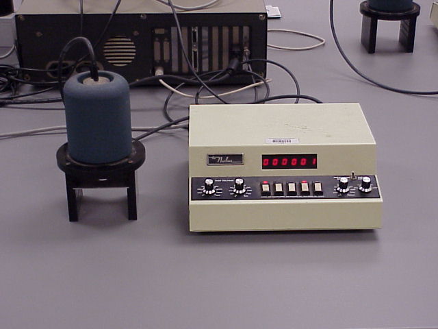
Below is a picture of a Geiger Counter in our lab. The tube and counter are shown. On the counter, the user can set the counting time. The counter options include start, stop and reset. The display shows the number of radiation particles recorded during the counting time.

The virtual Geiger counter operates similar to the real one. Click here for the Virtual Geiger Counter. The Geiger counter has two sample holders. In each sample holder you can pick either an empty holder, ¹³⁷Cs (2 μCi), or ⁵⁴Mn (5 mCi). In the left holder you also have as an option the short lived isotope ^137mBa as a sample. The detector has a dead time, and there is background radiation. The buttons are similar to a real Geiger counter. To operate: set the counting time and click the "start" button. Counting stops after the counting time. Then clear the counter with the "reset" button. To record counts from the ^137mBa sample, you need to select the sample and click on "squeeze out Ba". Squeezing out the sample refreshes the Ba source, which has a short half life. The Ba source is only activated when it is in the sample holder and squeezed.

Some experiments that can be done:

1. Dead time measurement: Measurement of the detector's dead time using the two source method.
2. Statistics of Nuclear Decay: Examine if the detector's counts follow a Poisson distribution.
3. Efficiency measurement of the detector
4. Half-life of ^137mBa: Take data on ^137mBa and determine its half-life. Remember to account for background and dead time.

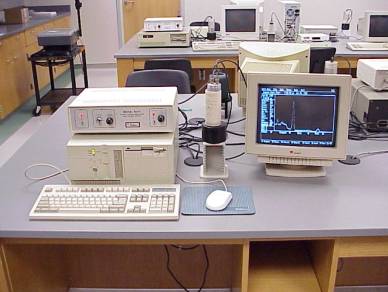
Below is a picture of our NaI detector / Multi-Channel-Analyzer (MCA) setup. The complete setup includes: the NaI detector with photomultiplier tube, Power supply and amplifier box, and computer with MCA card.

For each gamma-detector experiment described below, the MCA screen is displayed with different sample options. Pick a sample from the list and click on "Collect Data", which displays the spectrum. The total number of channels is 1024, and the "pan" buttons allows you to pan left or right the amounts indicated. There are two cursers. The channel number and counts for each curser are displayed underneath the screen.
Single Peak Fitting: The code allows the user to perform Gaussian peak fitting as follows: first set the left cursor (blue) with the "left cursor" button(s). Then set the right cursor using the "Width" button(s). Then click on "initial try" after Single Peak Fit. Click on "auto Fit" to improve the fit. Each time "auto Fit" is clicked a grid search is performed to minimize the total χ². Keep clicking on "auto fit" until the total χ² stops decreasing. The best-fit Gaussian parameters are displayed on the screen.
Double Peak Fitting: The code also allows for fitting two overlapping Gaussian peaks. Arrange the cursors so that they enclose both peaks. Then click on "initial try" after "Double Peak Fit". Two peaks should be displayed under the larger peak. Change the value in the box for "Center 2" to match the second peak. Then click on "manual Try". If the peaks are pretty close, then click on "auto fit" till the χ² stops decreasing.

To get an idea of how the detector works in the lab click on MCA Detector. In this app, the counts "grow" in time in each channel similar to how the detector collects data in the lab. For the MCA experiments below, the data was taken in the lab and is displayed in the programs.

For information on the NaI detector experiments and the grid search, see "Data Analysis in the Undergraduate Nuclear Laboratory", Byron Curry, Dave Riggins, and P. B. Siegel, Am. J. Phys. 63, 71- 76 (January 1995).

Energy Calibration Experiment

To run the code, click on gamma detector (Calibration) You will see the MCA screen with 800 channels. You can pan to the right to see the last 200 channels. The samples include three standards and an unknown. The unknown is a single isotope which gives off 2 gamma's when it decays. Your goal is to determine the photopeak energies and the identity of the unknown.

The energy of the detected gamma is (approximately) proportional to the channel number. Use the standards listed below:

to determine the parameters of the linear relationship between channel number and energy. Then find the channel numbers of the photopeaks of the unknown, determine their energies from your calibration line, and interpolate to find the gamma energies of the unknown.

Measuring the activity of a Salt Substitute (KCl)

The Salt substitute was bought in a supermarket, and is pure KCl. To run the experiment, click on Salt Sample Activity You will see the MCA screen with 1024 channels. The relevant data on the calibration standards are listed in the table below:

All the calibration samples were recorded for two minutes counting time. Note that the calibration was done 5 years ago, so you need to account for the natural decay of the calibration standards. In addition to these calibration samples, the Salt Substitute sample and a background were counted for two hours. By background we mean that the detector was on for 2 hours with no sample present. All samples have approximately the same source-detector geometry. Your goal is to determine the activity in decays/sec of the Salt sample. An isotope of potassium, ⁴⁰K, is radioactive and emits a gamma with an energy of 1460 KeV and a yield of 0.1068. One approach you can take is to first find the efficiency of the detector at the energies 662KeV, 511KeV, 1275KeV, 570KeV and 1063 KeV of the three standards. Make a graph of your results, and extrapolate to estimate the efficiency of the detector at 1460 KeV, which is the energy of the gamma emitted by K⁴⁰. Using the counts under the 1460 KeV peak from the KCl sample, you can determine the activity of the sample. Remember to subtract the background ⁴⁰K radiation, and to use the yield values in table above.

Attenuation of Gamma radiation in Lead Experiment

The program gamma attenuation in lead experiment contains gamma spectrum data with different absorbers between the source and detector. The source used was ¹³⁷Cs, which gives off a gamma with energy 662 KeV and an x-ray with energy of 32 KeV. The 662 KeV photopeak is located near channel number 278. The data are taken with lead absorbers of various thickness to attenuate the gamma particles. The lead absorbers block the x-ray completely, but the 662 KeV gamma particles do pass through. All data were taken with the same source-detector geometry.

Your goal in the experiment is to see if the attenuation is exponential with absorber thickness, and if so, determine the linear mass attenuation coefficient for the 662 KeV gamma for lead . Measure the number of gamma particles that pass through the lead for the absorbers given. Use Gaussian curve fitting to determine the area under the photopeak.

The data are as follows:

Collection time was two minutes in each case. Tables for the literature values of the attenuation coefficients can be found in tables.

Attenuation of X-ray radiation in Aluminum Experiment

The program x-ray attenuation in aluminum experiment contains spectrum data with different absorbers between the source and detector. The source used was ¹³⁷Cs, which gives off a gamma with energy 662 KeV and an x-ray with energy of 32 KeV. The photopeak of the x-ray is around channel 90. The data are taken with aluminum absorbers of various thickness to attenuate the radiation. The aluminum absorbers do attenuate the 32 KeV x-ray. All data were taken with the same source-detector geometry.

Your goal in the experiment is to see if the attenuation is exponential with absorber thickness, and if so, determine the linear mass attenuation coefficient for the 32 KeV x-ray for aluminum. As with the previous experiment, measure the number of x-rays that pass through the aluminum for the absorbers given. Use Gaussian curve fitting to determine the area under the photopeak.

The data, for a two minute counting time, are as follows:

Tables for the literature values of the attenuation coefficients can be found in tables. Note: the amplification has been doubled from the previous 662 KeV data, so the x-ray peak at around channel number 91 can be more clearly measured.

Soil Sample Analysis using the NaI gamma detector

As a final experiment with our NaI gamma detector, we analyze a soil sample. The experiment is described in exp5nai.pdf. The goal is to determine the activity of the ²³⁸U series, the ²³²Th series, and the percent by weight of potassium in the soil. There are many gammas emitted from these natural isotopes. Although the NaI detector's FWHM is only 6% at 662 KeV, we are able to resolve one gamma from each series: from the ²³⁸U series a gamma at 1764 KeV, from the ²³²Th series a gamma at 2614 KeV, and for potassium a gamma at 1460 KeV. The important gammas and their yields are listed in the table below:

Since these gammas are at different energies, the first thing we need to do is to determine the dependence of the detectors efficiency on the gamma's energy. This is done using standard disk sources. We use the following ansatz to relate the count rate C to the activity A of the isotope:

Below we show our high resolution Germanium detector from Canberra. The complete setup includes the detector with liquid nitrogen cooling, power supply, amplifier and a computer with a multi-channel analyzer card. There are 8192 channels.

The germanium detector is similar to the NaI detector, except that the resulution is significantly better and the data consist of 8192 channels. The computer program is similar to the NaI program. The screen displays 800 channels at a time. To move left or right through the complete spectrum, use the pan buttons as before. Gaussian peak fitting also works the same way as with the NaI detector program.

Environmental Sample Experiment

Click on Environmental Sample Experiment for the germanium detector for soil and rock analysis. There are three goals that you can have: (1) to determine the radioactive isotope content of the soil sample, (2) to determine the natural abundance of ²³⁵U in the rock sample, and (3) determine the age of the brazil nuts. Information about the gamma decay series for the natural occurring isotopes can be found in tables. Information about the characteristic x-rays given off by the various daughter isotopes can also be found in tables. These exercises may be difficult. We have written a program to assist in the analysis which you might find useful: soilfit.html To assist in the calculations, see "Gamma Spectroscopy of Environmental Samples", P.B. Siegel, Am. J. Phys. 81, 381-388 (May 2013).

Data for Ge detector:

1. The file "Calibration" is a spectra obtained by counting for a few minute with calibration samples. The Calibration samples are: ¹³⁷Cs, ²²Na, ⁶⁰Co, and ²⁰⁷Bi. Note that the photopeak for ¹³⁷Cs, 661.64 KeV, isaround channel 3278.
2. The file bkrd20hr is a spectra obtained by counting for 20 hours with no sample present. It is a "background" recording.
3. The file "Soil Sample" is a spectra obtained by counting for 20 hours with a soil sample from Oakhills. The mass of the sample is 4305 grams.
4. The file "Soil Sample with 112.7 gms of KCl" is the same soil sample from Oakhills with 112.7 grams of KCl salt mixed in uniformly. This file will assist in determine the efficiency for our detector-source setup, since the detector-source geometry is the same as the soil sample.
5. The file "Brazil nuts" is a spectra obtained by counting for 20 hours with a sample of Brazil Nuts. The mass of the nuts is 2000 grams, and the detector-source geometry is the same as the soil sample.
6. The file "desert rock" is a spectra obtained by counting a rock, which contains a significant amount of uranium.

This spectrometer measures optical spectra from wavelengths 200-1100 nanometers. The Ocean Optics Spectrometer measures the intensity (classical) of the radiation. Here, we are not counting photons as was done with the gamma detectors. The intensity in each "channel" is not an integer, and does not necessarily obey Poisson statistics. The shape of the peaks are not necessarily Gaussian. However, the peaks are close enough to a Gaussian shape that we can fit them as we did with the gamma spectrometers. To run the experiments click on: Ocean Optics Spectrometer. Below are some experiments that we will perform.

1. Wavelength Calibration
The virtual optical spectrometer contains numerous hydrogen and helium spectra taken with different collection times. The collection time for each spectra is listed in the select box. The hydrogen spectra are used to calibrate the detector. For calibration standards, we use the Balmer lines listed below:

2. Helium Spectrum Analysis
Measure as many spectral lines as you can for helium. Then look for patterns in ΔE_ji, which is defined and explained in the experiment description: Experiment 6.

1. Liquid Scintillation Detector is a program that simulates our 2000 channel liquid scintillation detector. You can choose four different samples: empty(none), ³H (tritium), ¹⁴C, or an "unknown". You can also choose different counting times. Both the ³H and the ¹⁴C samples had an activity of 100000 dpm when calibrated 17 years ago. Your goals are to:

• Determine the counting efficiency for both ³H and ¹⁴C.
• Determine what the unknown sample is.

2. RIA Calibration and RIA Experiment are two programs that simulate our radioimmunoassay experiments. Your goal in the experiment is to determine how the concentration of the hormone aldosterone changes in the blood of an animal over time after the injection of angiotensin II. The times after injection are 0, 2, 4, 6, and 8 hours. To carry out the experiment you need to first calibrate the assay technique with the program RIA Calibration. Once you have a calibration curve, you can run the program RIA Experiment to determine the aldosterone concentration over time.

3. Transport Assay Experiment is a program which simulates our Gaba transport assay experiment. Your goal is to determine the GABA transport rate as a function of the GABA concentration for both the control and the GAT3-expressing cell. The program allows you to input the "cold" Gaba concentration (from 0 to 500 micro-molar) added to the incubation solution. A pull down menu allows you to choose which sample is placed in the liquid scintillation detector: 10 micro-liters of solution, the control cell, or the GAT3-expressing cell. All incubation solutions contain the same amount of "hot" GABA. For more information on the experiment, see experiment 9 in our lecture notes: Radiation Biology Lecture Notes.